From Zero to Driverless Race Car with Deep Learning
This post is based on the following talk.
Abstract:
Learn how to train a driverless car to drive around a simulated race track using end-to-end deep learning — from camera images to steering commands. Key techniques used include deep neural networks, data augmentation, and transfer learning. This was a course project, so I'll introduce the key ideas and talk about the practical steps needed to get it working. You'll also see a lot of very dangerous driving.
Introduction
Today I’m going to talk about how to build a driverless race car using deep learning.
I should start by saying that this was a personal project, but it does have a connection to my work. By day, I’m CTO of Overleaf, the online LaTeX editor. Overleaf now has over three million users, and the first two, namely my co-founder and I, were driverless car researchers! We started Overleaf while we were working on the Heathrow Pod, which was the world’s first driverless taxi system. It launched in 2011, and it’s still running, so if you ever have some time at London’s Heathrow Airport, you should take a ride on the pods out to business parking and back to Terminal 5.

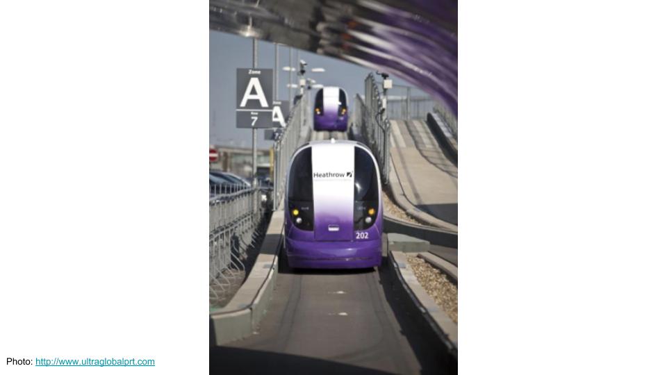
The key thing allowed us to put driverless taxis into active service way back in 2011 is that the taxis run on their own roads. It’s a closed system, and we used a fairly traditional systems engineering approach to design and build the system and prove that it was safe.
Nowadays most driverless car research is about how we get them to work safely on public roads, where we need to worry about human drivers and pedestrians and cyclists and traffic lights and stop signs, and lots of other messy things.
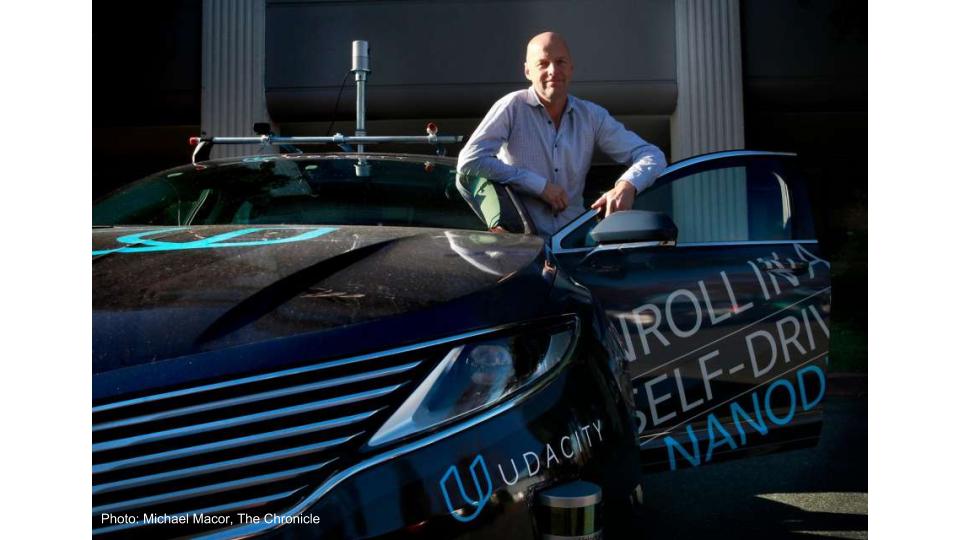
One of the pioneers in this area is Sebastian Thrun, who was a professor at Stanford and leader of the winning team in the 2005 DARPA Grand Challenge, which in many ways inaugurated the modern driverless car era. He later left to start Udacity, one of the leading MOOC providers, and they launched a driverless car course in 2016 1, the Self-Driving Car Engineer nano-degree. It sounded great and with my copious free time (!) I enrolled.
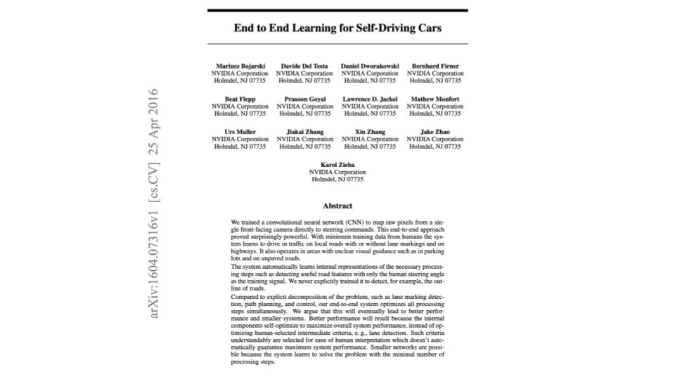
This talk is based on one of the labs in that course, which is in turn based on a 2016 paper from NVIDIA, called End-to-End Learning for Self-Driving Cars. What the NVIDIA team showed is that it’s possible to take images from a front-mounted camera on a car, feed them into a convolutional neural network, which we’ll talk about, and have it produce steering commands to drive the car. So, just like you look at the road ahead and decide whether you need to steer left or right, they did the same thing with a neural network.
What’s remarkable about this is that it’s very different from the systems engineering approach that we usually take in driverless car engineering. In that approach we break the overall problem of driving the car down into lots of subproblems, such as object detection, object classification, mapping, planning, etc., and have different subsystems responsible for each of those subproblems. The subsystems are then connected up to make the whole system. Here, however, we’re just going to train one big monolithic neural network, which will somehow drive the car. It feels a bit like magic.
Our task for this lab was to reproduce this magic, and this talk follows steps I went through to do so, which were broadly:
- Collect training data in a simulator by driving around the track manually.
- Train a deep neural network using the camera images and steering angles.
- Use the network to drive the car around the track (also in simulation).
In the middle, I’m going to handwave quite a lot about some of the theory. You may wish to skip that part if you are already familiar with convolutional neural networks.
Collecting Training Data
The first thing we need to do is collect training data by driving the car around in the simulator. We’re going to train the neural network to imitate me, so here I am trying to drive mostly in the center of the road, like we want the neural network to do.
You can see in the top right a ‘recording’ sign, which means that we’re recording the camera images and my steering angle for each frame, 10 times each second.
You might notice that I’m not very good at this. One of the key reasons is that the only way to steer the car is with the left and right arrow keys. So, the first thing we need to do is take my raw steering inputs and clean them up by smoothing them.
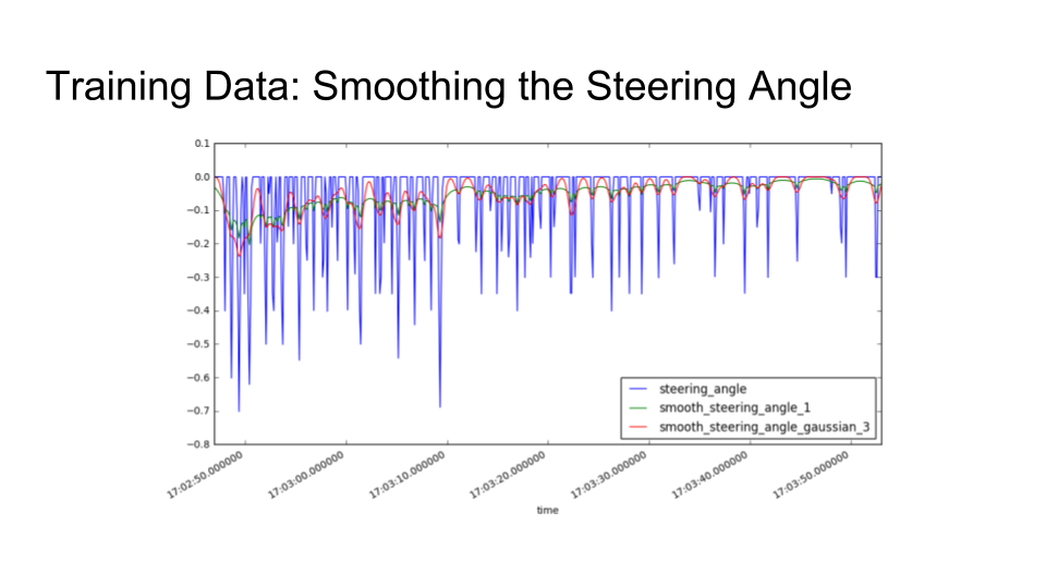
The spiky blue line is the raw steering input from me pressing the arrow keys. The green and red lines are the results of applying exponential and Gaussian smoothing, respectively. I tried both kinds of smoothing, and the Gaussian smoothing turned out to work better when actually driving the car.
The next hurdle to overcome in this training process is that if I only show the car how to drive in the center of the road, it will never gain any experience of what to do if it ever finds itself off-center. We can solve this problem by recording recoveries in training, in which I stop the recording, drive off to the side of the road, start recording, and then drive back into the middle:
By doing this, we teach the car how to get back to the center of the road, hopefully without teaching it too much about driving off the road.
After driving around the track several times in both directions and doing recoveries, I ended up with about 11 thousand frames of training data: 2
| Dataset | Rows (Frames) |
|---|---|
| Normal | 5,273 |
| Recoveries | 6,037 |
| Total | 11,310 |
That is in some sense quite a lot, but in the world of deep learning, it is not very much at all, and I think we would struggle to train a network from scratch using just these data. To get around that, we’ll use a technique called transfer learning.
Transfer Learning
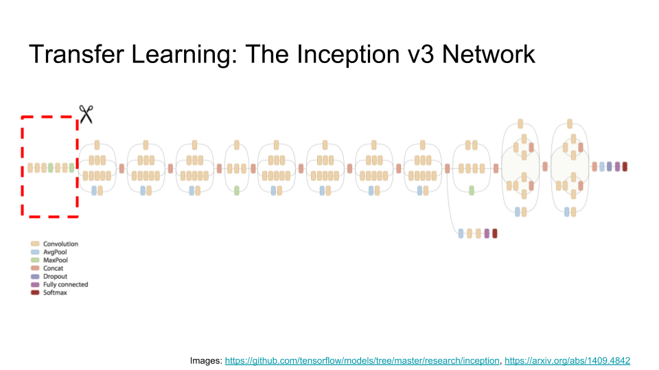
Transfer learning means that we take someone else’s network that they have already trained for some other task, extract a little bit of it, and repurpose it for our task.
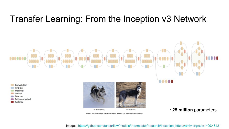
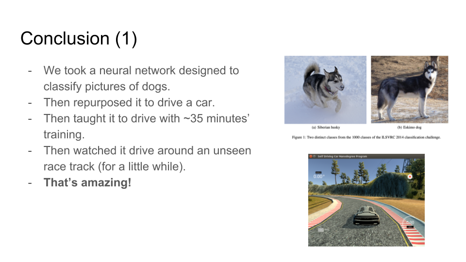
Here we’re going to use the Inception v3 network, which was trained by Google for an image classification competition. It takes as input an image, runs lots of computations, and outputs the class of the image — that is, what kind of thing the image shows. If you feed in the image on the left, it will tell you that that is a Siberian Husky, and if you feed in the image on the right, it will tell you that that is an Eskimo Dog. (It is interesting to note that some of the classifications are quite fine; I’m not sure I could tell the difference!)
The Inception network is a very large — it has over 25 million parameters, which Google has trained with considerable effort and expense. So, how would we go about building on the work that they’ve done? The answer is surprisingly simple: we ‘lobotomize’ the network and just take the first few layers (indicated by the red dashed box below).
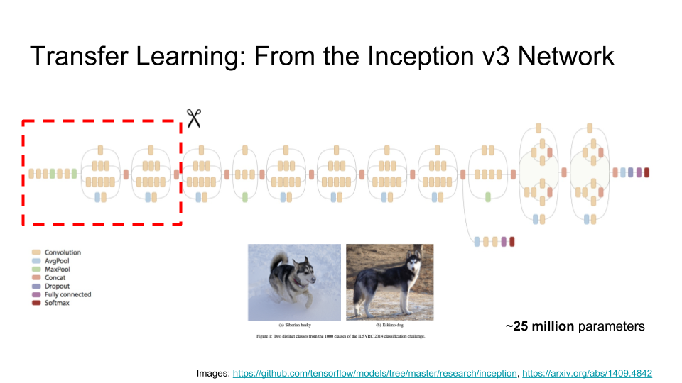
The reason this works is that these first few layers of the network, 44 layers to be precise, turn out to be relatively generic image processing stuff — different kinds of edge detectors, for example. It is the later stages of the full Inception network that encode the difference between Siberian Huskies and Eskimo Dogs, and all of the other image classes, which we don’t need. So, for our application, we’re just going to tack a relatively small neural network on to the end of our Inception prefix network:
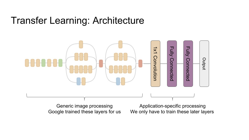
That means that we only have to train these last few layers ourselves, leaving the pre-trained Inception prefix network alone, so we can hopefully get away with much less training data than if we started from scratch.
I should add the architecture of our last three layers was chosen after some trial and error with even simpler architectures, and this was the simplest one that seemed to work.
Convolutional Neural Networks
So, how does this network actually work? This is where I will talk about some of the theory. To build a convolutional neural network, which is the kind of deep neural network that this is, we need three basic building blocks:
- Convolution
- Resizing (in particular making the images smaller)
- Activation Functions
Let’s take each of these things in turn. I’m going to use this camera frame as an example:
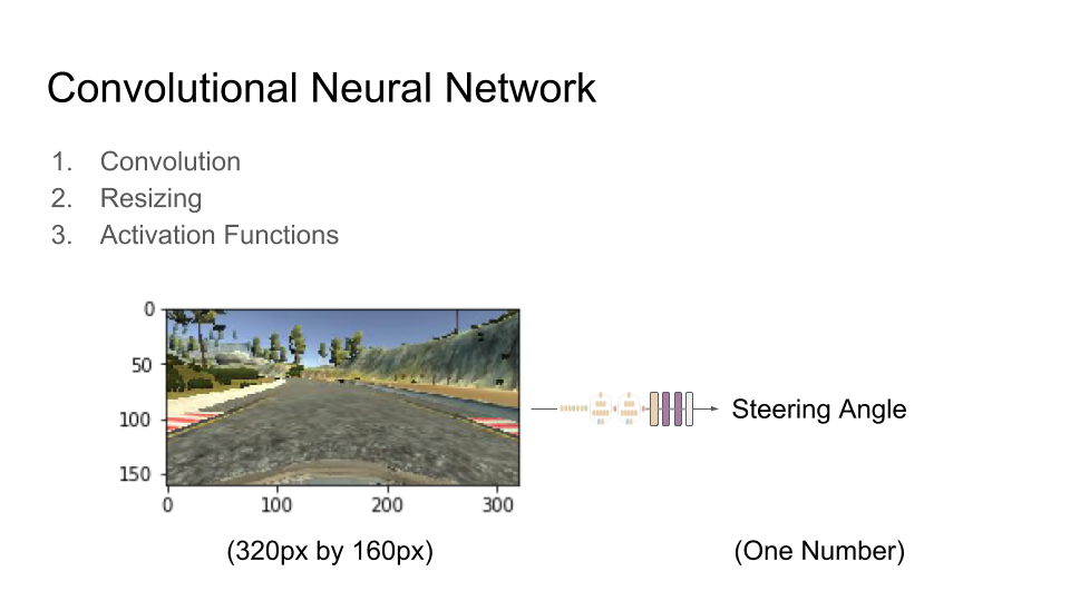
One way to look at it is that our overall aim for this network is to go from a camera frame at 320 by 160 pixels down to a single number, which is the steering angle that the car should apply when it sees this image.
Let’s start with our first building block, convolution. Convolution is a simple idea but also a very general one. To use it, we define what is called a kernel (it has many names, but I will call it a kernel), which is a small matrix of numbers. Here we’ll use a 3 pixel by 3 pixel kernel.
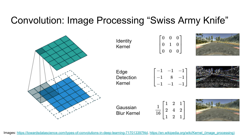
We start by lining up our 3 pixel by 3 pixel kernel with the 3 pixel by 3 pixel patch in the top left corn of the image. We then multiply each pixel in the image with the corresponding value from the kernel and add them up to give us the first pixel in the output image 3. Then we slide our kernel over the rest of the pixels in the input image, pixel by pixel, each time yielding one more pixel in the output image: 4
This operation is very simple and can be done efficiently, but it is also very powerful. If you use a program like Photoshop, most of the tools in the image filters menu will be using a convolution under the hood, each using a different kernel. The identity kernel is not very interesting, because it just copies the input to the output, but we can also choose kernels for edge detection, blurs, sharpens, and much more.
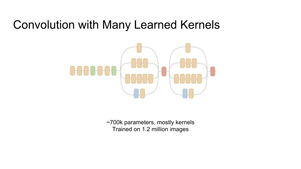
To use convolution in a neural network, the key insight is that instead of very carefully engineering these kernels ourselves, we let them be learned from the training data. And we let the network learn a lot of different kernels. The prefix of the Inception network that we’re using has about 700 thousand parameters, many which are are kernel parameters, which Google has trained using 1.2 million images.
When we run convolutions with so many kernels, we basically take one input image and produce lots of output images — one for each kernel. If we were to keep adding more and more images, we would run out of memory, so we also need our next building block: resizing.
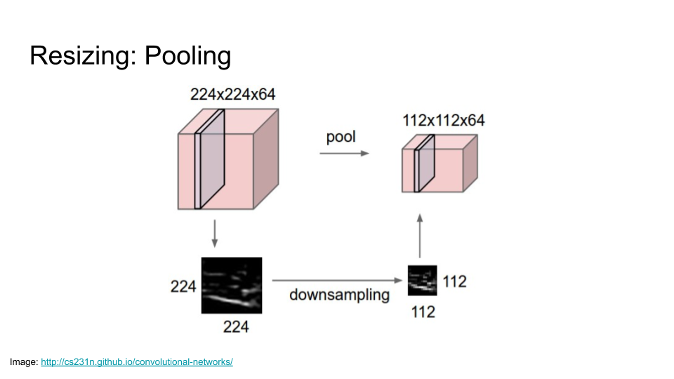
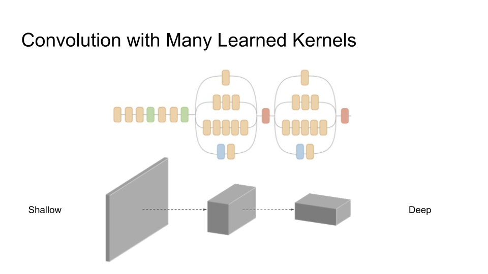
This does what it says on the tin: every few convolutions, we resize the image to make it smaller. There are lots of ways of doing this, such as max pooling.
When we resize, we lose some spatial resolution, but we gain depth. It lets us take our flat input image, and by repeated convolutions and resizing, get to a sausage shaped ‘image’ that is lower resolution but also deeper. The network gains, in some handwavy sense, understanding with this depth — it started out with a patch of image that was just pixels, and now it has mapped those pixels into a set of features that can carry more meaning to help it solve the task at hand.
Our final building block is the Activation Function, which is where the ‘neural’ in ‘neural network’ comes from.
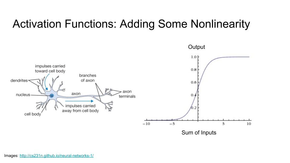
A real neuron is an incredibly complicated thing with amazing dynamics and lots of interesting behaviors, but we are going to model it in a very simple way. Essentially, it has dendrites, which are ‘inputs’ connected to upstream neurons, and if those inputs add up to at least some threshold, this neuron is going to activate and send a signal through its axon to downstream neurons.
Mathematically, we can represent this as a very simple squashing function. If the sum of the inputs is negative, it outputs a value near zero, which means that it is not activated. If the sum of the inputs is positive, it returns a value near one, which means it is activated.
These three building blocks are all we need. We just repeat them over and over again. It’s worth noting, however, that convolution (of the kind used here) is a linear operation. If it were not for the little bits of nonlinearity that we get from (most kinds of) resizing and the activation function, the composition of convolutions would collapse down to one big linear function. However, once we add these relatively tame non-linearities into the mix, we go from being able to represent only linear functions to being able to approximate any function, which is pretty amazing.
Completing the Network
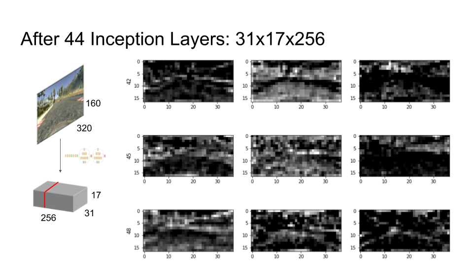
So, that’s the end of my theory bit. Let’s see what it does in practice using our example camera image. When we feed it through the first 44 layers of the Inception network, we get back 256 greyscale ‘feature images’. The width and height of each feature image are about a factor of 10 smaller than the input image, but there are many more of them — as noted above, the output is much smaller and deeper than the input.
Here are nine feature images, starting mostly at random from feature image number 42, out of our stack of 256. Each image shows one of the responses that the network gives to our example input image. A light pixel means that the neuron at that point in the feature image is activated — it’s responding to some characteristic of the corresponding part of the input image. A dark pixel means it isn’t activated.
If we overlay the response with the input image, it becomes easier for us to interpret what they’re responding to:
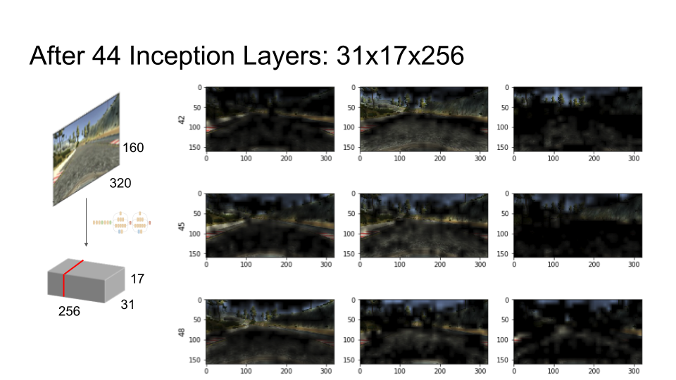
In feature image number 42 (top left), for example, we can see some neurons responding fairly strongly to the edges of the road. When driving, it is pretty important to know where the edges of the road are, so this feature image may be useful. Number 43 (top center) seems to be responding to the road surface, which may be similarly useful. It’s also picking up some of the background, but we can also see that number 48 (middle right) is responding mainly to the background. So, it seems like some combination of these feature images would give us useful information.
It’s important to note that we didn’t tell this part of the network how to find features that might be helpful for our task. In fact, this part of the network was trained by Google for a completely different task, namely image classification, but it seems to have some features that look like they may be useful for our task, which is encouraging.
This brings us back to the bit of the network that we actually train, which are the three layers that we’ve added at the end.
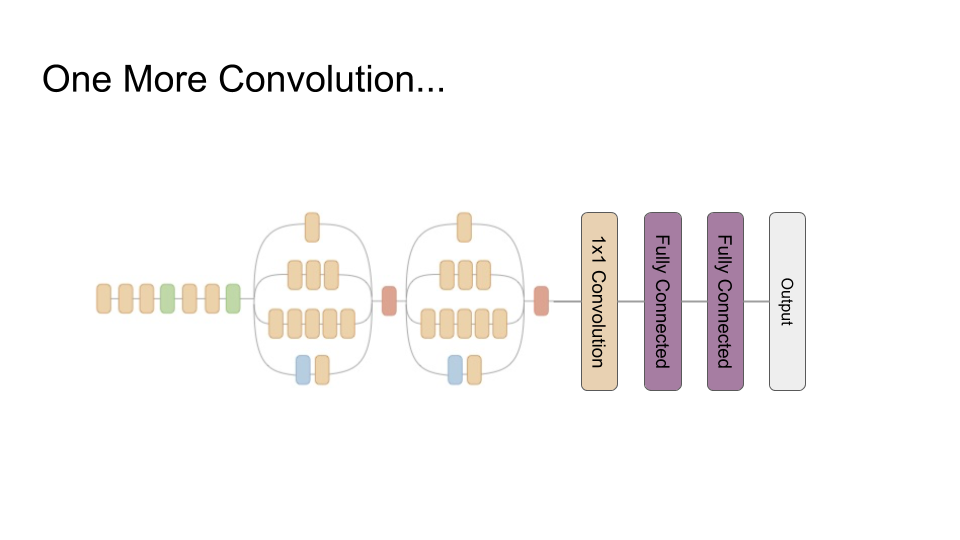
Our first layer is another convolution. This is a ‘one by one’ convolution, which means a kernel size of 1 pixel by 1 pixel. A 1x1 convolution picks a set number of linear combinations of its input feature images; it is often used for dimensionality reduction. This architectural choice is motivated by the discussion above about how some linear combination of features images 42, 43 and 48 seems like it might be pretty good at finding the road — we want to let the network pick the most useful combinations of the 256 feature images from above.
In this example, we’ll pick 64 linear combinations of the 256 features. Here are some new feature images after that 1x1 convolution. They look similar, but they are generally smoother and brighter than the feature images before the 1x1 convolution.
![]()
![]()
Again we can see some features responding strongly to the edges of the road, for example feature image number 45 (out of the 64 new feature images this time).
Finally, we have two fully connected layers. From now on, we won’t be able to visualise the results so easily, because we flatten all of the outputs from the convolution into one large list of numbers. A fully connected layer then computes a set number of linear combinations of all of those numbers.
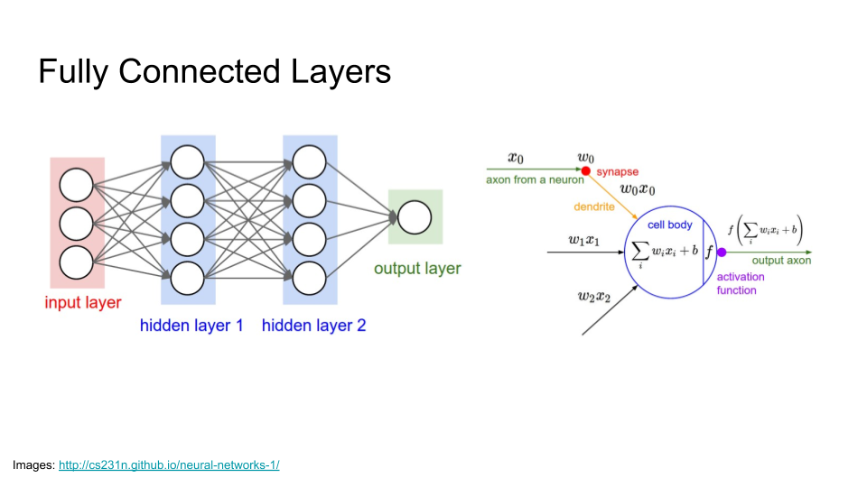
The diagram on the right shows a schematic for one of those linear combinations — that is, one neuron – in one fully connected layer. A fully connected layer consists of many such neurons, each connected to all of the outputs of the previous layer. Here the weights we train are the wi, and the inputs are the xi. And again we apply an activation function, here denoted f, to each neuron to introduce some nonlinearity, so our two fully connected layers don’t just collapse down into one big linear function.
The outputs of the first fully connected layer feed into the second fully connected layer, and the output of the second fully connected layer is, at last, our steering angle! With our network architecture set out, we are ready to start training.
Time to Train
Well, almost ready. Even just for three layers that we need to train, there are quite a few hyperparameters that we need to set before we can fully define the network and the training scenario. How many kernels should we use in our 1x1 convolutions? How large should each fully connected layer be? What kind of smoothing should we do on the steering angle? And many more.
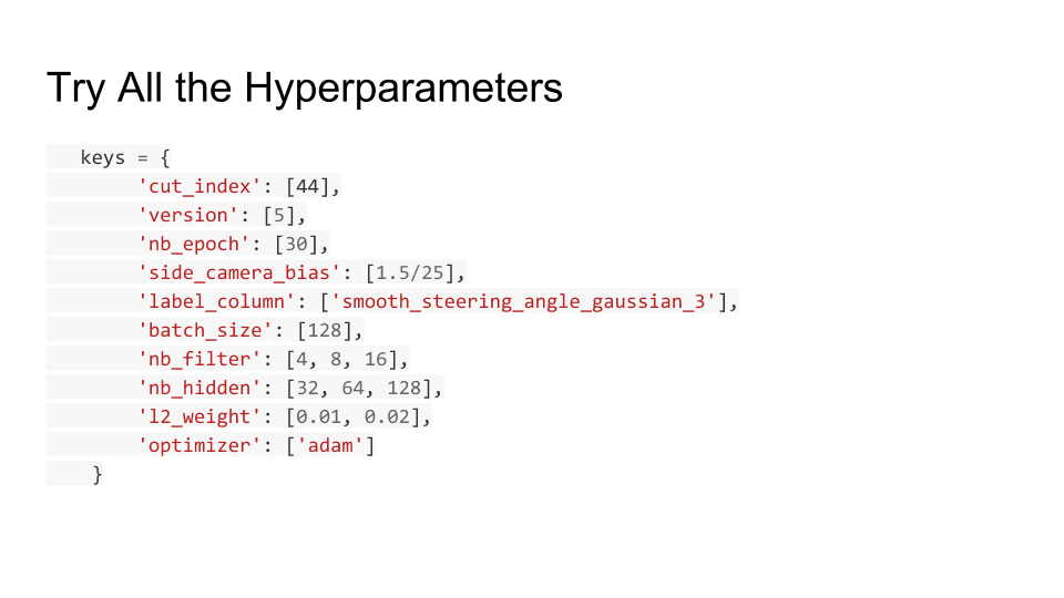
There are smart ways to search hyperparameters, but in this case I just tried all possible combinations in a large grid search. It takes a while to run the whole grid, but it’s just computation — set it off before bed, and by the time you get home from work, new data are waiting.
Each point in the grid gives one network to train and evaluate. Then we can evaluate the performance of each of the networks to choose the best hyperparameter settings.
Fortunately, the actual training is made very easy by great libraries, such as Keras. Here’s an example of the Keras training output for one of the networks:
Layer (type)                     Output Shape          Param #     Connected to
====================================================================================================
convolution2d_1 (Convolution2D)  (None, 17, 37, 64)    16448       convolution2d_input_1[0][0]
____________________________________________________________________________________________________
flatten_1 (Flatten)              (None, 40256)         0           convolution2d_1[0][0]
____________________________________________________________________________________________________
dense_1 (Dense)                  (None, 32)            1288224     flatten_1[0][0]
____________________________________________________________________________________________________
dense_2 (Dense)                  (None, 1)             33          dense_1[0][0]
====================================================================================================
Total params: 1304705
____________________________________________________________________________________________________
Epoch 1/30
27144/27144 [==============================] - 160s - loss: 79.0047 - val_loss: 0.0780
Epoch 2/30
27144/27144 [==============================] - 147s - loss: 25.4130 - val_loss: 0.0692
Epoch 3/30
27144/27144 [==============================] - 148s - loss: 8.4912 - val_loss: 0.0670
Epoch 4/30
27144/27144 [==============================] - 148s - loss: 2.9383 - val_loss: 0.0638
…
Epoch 12/30
27144/27144 [==============================] - 148s - loss: 0.0851 - val_loss: 0.0572
Epoch 13/30
27144/27144 [==============================] - 148s - loss: 0.0785 - val_loss: 0.0568
Epoch 14/30
27144/27144 [==============================] - 148s - loss: 0.0802 - val_loss: 0.0546
Epoch 15/30
27144/27144 [==============================] - 147s - loss: 0.0769 - val_loss: 0.0569
Epoch 16/30
27144/27144 [==============================] - 147s - loss: 0.0793 - val_loss: 0.0560
Epoch 17/30
27144/27144 [==============================] - 148s - loss: 0.0832 - val_loss: 0.0574
There’s a lot going on in this output, and I’d like to remark on a few things. At the start of the output, we have Keras’s summary of the model we’re training, which includes numbers of parameters to fit. Remember that we’re keeping the layers from the Inception network that Google trained completely fixed, so we’re only worried about training our three layers at the end of the network. 5
In the second section, we have the training progress, which Keras prints as it goes. I’ve split the training data I collected into a training set (80%) and a validation set (20%). 6 At each Epoch, Keras reports the mean absolute error in the network’s predictions on the training set (the loss) and the validation set (the val_loss).
For each of our three layers, training starts with randomly initialized weights. As you might expect, the initial loss with random weights is pretty terrible, starting at around 79 7. However, Keras uses that loss to refine the weights for the next epoch, feeds the training set through again, and sure enough the loss drops with each successive epoch. After 17 epochs, the loss is orders of magnitude lower, at 0.08. Training stops when the validation set loss, val_loss starts to increase — to run more epochs would likely lead to overfitting.
Run the Model with Lowest Validation Loss!
So, after repeating that training process on hundreds of networks for all our various hyperparameters, let’s hook up the network with the best validation set loss to the car and see how it drives!
We put the simulator into autonomous mode, then the car starts moving. I haven’t talked about throttle control, but basically it sets the throttle to keep the car at about 10mph in this case.
We can see the car weaving, and then correcting, but it overcorrects, and eventually it runs off the road and crashes. Still, it is not a bad start — it was clearly trying to stay on the road, which is encouraging.
Try Lots of Things…
And so the debugging begins. There were lots of arbitrary decisions not in my initial grid of hyperparameters, so I started by adding many more to the grid. For example:
- Different loss functions — how should we measure the error? I tried mean squared error and mean absolute error; the latter seemed a bit better.
- Different activation functions — I tried sigmoid, tanh and ReLU; tanh seemed a bit better.
- Different regularization — penalizing the weights so that they do not become too large is a common technique to avoid overfitting, and I tried several different L2-regularization weights.
- Different distributions for initial weights (reduce variance of Normal) — this did solve some convergence problems during training.
- Different layer sizes — how many neurons in each hidden layer?
- Different network architectures — try adding more layers? Or fewer layers?
However, none of the things I tried really moved the needle. After thrashing around for a few days without getting anywhere fast, I stopped fiddling with the neural network and added a print statement to the control loop. That quickly revealed the actual problem:
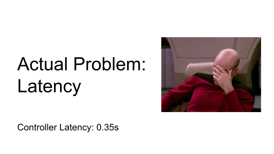
The controller was spending too much time processing each frame, so it was only actually able to steer about three times per second. If you imagine trying to steer, but you can only touch the wheel three times a second, it does seem pretty tough. Further investigation revealed that it was spending most of its time in the Inception prefix layers. One solution would have been to buy a faster laptop. However, it turned out that it was possible to use fewer inception layers, in particular the first 12 layers, instead of the first 44 (it looks like 7 in the diagram, but some are not visible):
With Lower Latency
Let’s see how it does with lower latency (about 0.1s instead of 0.35s):
It now does much better. I’ve sped up the video, because it makes it much further. The weaving is much reduced, and it’s staying mostly in the middle. It’s not following a great ‘racing line’, but that’s probably because I didn’t follow a great racing line when I was training it.
Eventually it gets to a turn where there are some trees ahead of it, and it doesn’t make the turn. Still, progress!
The resolution for this problem was basically to add more training data — I drove around that corner a few more times, and eventually it learned to make it. At around the same time, Udacity released a bunch of training data from someone who had a steering wheel, instead of having to do the arrow keys and smoothing, so I added that in too.
I also did some augmentation with the training data, which in retrospect was fairly obvious: you can mirror every image in your original training set and negate the steering angle, and you have another training example.
The Final Result
With all this additional training data, the network managed the following:
I changed the throttle control to let it drive at 30mph, which was the cap in this version of the Udacity simulator, so it’s going quite a bit faster. You can still see some ‘shimmy’ but it is no longer crashing. Success!
Does it Generalize?
So, we’ve seen that for this race track, we can train the network and make it go around. What if we put it on a totally different race track? Fortunately Udacity provided just a second track in the simulator, so let’s try it out. Note that this is exactly the same network as in the previous video, and it has not seen any part of this new track in its training data.
Behold, it drives! Again it shows sensitivity to trees, with a near miss at 0:24 and eventually a crash, both with trees in its field of view. Still, considering that this is a very simple network, as neural networks go, and it hasn’t had a huge amount of training, the fact that it does this well on an unseen track, albeit one in the same simulator, is I think pretty good.
Conclusions
In this post we:
- Took a neural network designed to classify pictures of dogs.
- Repurposed it to drive a car.
- Taught it to drive with ~35 minutes’ training.
- Watched it drive around an unseen race track (for a little while).
That’s amazing!
Moreover,
- In 2015, very few people would have even thought this was possible.
- In 2016, thousands of people like me were doing it in their spare time in an online course.
- In 2018, I mentored (very slightly) Josh, a high school student who did it all himself on an RC car with a Raspberry Pi.
That’s also amazing!

I prepared this talk for the 2018 Holtzbrinck Publishing Group AI Day. I would like to thank the organizers for giving me the impetus to finally write this talk and for providing the video.
The code for this project is open source.
If you’ve read this far, perhaps you should follow me on twitter, or maybe even join our team. :)
Footnotes
-
Udacity actually ran two driverless car courses. The first was CS373: Programming a Robotic Car, which I completed in 2012, and is still offered for free. The second was the Self Driving Car Engineer nano-degree. Both were great! ↩
-
The simulator actually takes three camera images in each frame, one on the left wing, one in the center, and one on the right wing. I also added the wing cameras to the training data, together with an empirically determined adjustment to the target steering angle to account for the different wing camera position. In that sense the number of examples is 33,930 (3 times 11,310), but it’s not clear how much these images add, since they are very similar to the central camera image. I didn’t have time to go into this in my talk. ↩
-
Here I have glossed over an important detail: the input image is a color image, so it actually has three channels, one each for red, green and blue (RGB). The convolutions in convolutional neural neworks operate on all of the channels in their input, so the kernels here should actually be thought of as three-dimensional kernels in this case — 3 pixels by 3 pixels by 3 channels. I did not have time to get into this detail in my talk (and drawing that would have been hard!). ↩
-
This image is from An Introduction to different Types of Convolutions in Deep Learning, by Paul-Louis Pröve, which is an excellent place to find out more about convolution. ↩
-
Because the Inception prefix layers remain fixed through training, a useful optimisation is to run the training data through the prefix network once and save the outputs. The saved outputs are then fed into the training process for the later layers many times. Quite a lot of the code is concerned with doing this, but it does make a big difference to training times. The output features from the prefix are usually called ‘bottleneck’ features, and the slides with example features from the Inception prefix network are taken from these bottleneck features. ↩
-
The eagle-eyed reader may notice that Keras reports 27,144 images in the training set, which is larger than the 11,310 points I reported in my table. See 2. The size of the training set is 80 percent of 11,310 samples times 3 frames per sample, which is 27,144. ↩
-
That is not 79 degrees; the angle has been scaled so that the range [-1, 1] corresponds to [-25˚, 25˚], so it is effectively doing donuts during the first training epoch. ↩