The Mathematics of 2048: Counting States by Exhaustive Enumeration
Updates
2017-12-11 This post was discussed on Hacker News.
This post is the third in a series. Next: Optimal Play with Markov Decision Processes.
So far in this series on the mathematics of 2048, we’ve seen that it takes at least 938.8 moves on average to win, and we’ve obtained some rough estimates on the number of possible states using combinatorics.
In this post, we will try to refine those estimates by simply counting every reachable state by brute force enumeration. There are many states, so this will require some computer science as well as mathematics. With efficient processing and storage of states, we’ll see that it is possible to enumerate all reachable states for 2x2 and 3x3 boards.
Enumeration of all states for the full game on a 4x4 board remains an open problem. I ran the code on an OVH HG-120 instance with 32 cores at 3.1GHz and 120GB RAM for one month, during which it enumerated 1.3 trillion states, which is a respectable half a million states per second, but that turns out to be nowhere near enough. At present, the best we we’ll be able to do on the 4x4 board is to enumerate all states for the game played up to the 64 tile.
Overall, the results show that the combinatorial estimates from the last post were substantial overestimates, as suspected. However, the state space for the full game is still very large. If a large nation state or tech company decided that 2048 was their top priority, which may not be the craziest thing that’s happened this year, I think they could probably finish the job.
The (research quality) code behind this article is open source, mainly in ruby and C++.
Counting States
Here a state captures a complete configuration of the board by specifying the value of the tile, if any, in each of the board’s cells. Our overall goal is to count all of the states that can actually occur in the game and no more. In the previous post, the estimates from (very basic) combinatorics counted many states that can’t actually occur in the game. By enumerating states systematically from each of the possible start states, we ensure that the states we count are actually reachable in play.
We also have some freedom in choosing which states are interesting enough to count. Because the game ends when we obtain a 2048 tile, we won’t care about where that tile is or what else is on the board, so we can condense all of the states with a 2048 tile into a special “win” state. Similarly, if we lose, we won’t care exactly how we lost; we can condense all of losing states into a special “lose” state.
Canonicalization and Symmetry
Many other non-interesting states that we’d like to avoid counting arise from the fact that some states are trivially related to each other by rotation or reflection. For example, in the game on a 2x2 board, the states
 and
and

are just mirror images — they are reflections through the vertical axis. If we swiped left in the first state, it would be essentially equivalent to swiping right in the second. We can therefore reduce the number of states we have to worry about by treating these states as equivalent. In general, the number of such equivalent states is the number of elements in the dihedral group for the square, \(D_4\), which is 8. For the first state above, these eight states are:

In this diagram, which is called a cycle graph, ⤴ denotes a rotation counterclockwise by 90° and ↔ denotes a reflection about the vertical axis. The three states at the top are obtained by one or more rotations; for example, ⤴² means two rotations of 90°, which add up to a rotation of 180°. The four states at the bottom are obtained by zero or more rotations followed by a reflection.
When the tiles in a state are arranged in a symmetrical pattern, the number of equivalent states may be less than 8, because the symmetry means that some of the states in the above diagram will be identical. For example, the state  has only four, because it is symmetric along the diagonal. However, particularly on 3x3 and 4x4 boards, states with symmetric arrangements of tiles are not so common, so overall we can expect to reduce the number of states we need to count by roughly a factor of 8 by choosing only one of these equivalent states as the canonical state.
States as Numbers
Which of the equivalent states should we choose as the canonical state? To answer this question, it will be helpful to think about states as numbers. We’ll also see that this has significant computational benefits in the appendices.
To write a state as a number, we can start in the top left and read the cells by rows; for each cell, we write a \(0\) digit if the cell is empty, and the digit \(i\) if the cell contains the \(2^i\) tile. For example, on a 2x2 board, the state
would be written as the number \(2310\), because \(4 = 2^2\), \(8 = 2^3\), \(2 = 2^1\), and the last cell is empty.
Since we’re only interested in numbers up to 2048, which is \(2^{11}\), we could in principle write any state as a number in base 12 (rather than base 10, as we are accustomed to). However, because computers run on binary numbers, it will be more convenient to think of each state as a number in base 16 — that is, hexadecimal. The state above would therefore be more properly written as 0x2310 for computer scientists or \(2310_{16}\) for mathematicians.
To find the canonical state, we simply try all eight possible rotations and reflections, convert the resulting states to numbers, and then pick the smallest one. For our example state, , the candidates and their corresponding numbers are:
| State | Number |
|---|---|
| 0x2310 |
| 0x3201 |
 | 0x1023 |
 | 0x2130 |
 | 0x0312 |
 | 0x1203 |
 | 0x0132 |
 | 0x3021 |
The state has the smallest number, 0x0132, so that is the canonical state for . In general, this system for choosing canonical states tends to put tiles with larger values toward the bottom right corner.
Enumeration
Now we’re ready to start enumerating states — it’s all computation from now on. The idea is to generate all possible (canonical) start states, then for each one try each possible move, then for each move generate all possible (canonical) successor states. In code (ruby) form, the basic algorithm for enumerating states looks like this:
def enumerate(board_size, max_exponent)
  # Open all of the possible canonicalized start states.
  opened = find_canonicalized_start_states(board_size)
  closed = Set[]

  while opened.any?
    # Treat opened as a stack, so this is a depth-first search.
    state = opened.pop

    # If we've already processed the state, or if this is
    # a win or lose state, there's nothing more to do for it.
    next if closed.member?(state)
    next if state.win?(max_exponent) || state.lose?

    # Process the state: open all of its possible canonicalized successors.
    [:left, :right, :up, :down].each do |direction|
      state.move(direction).random_successors.each do |successor|
        opened.push(successor.canonicalize)
      end
    end

    closed.add(state)
  end

  closed
end
The code for generating start states is here, and the code for the rest of the State methods, such as random_successors and canonicalize, is here.
If we run this code for the game on the 2x2 board played up to the 32 tile, which we’ve previously established is the highest tile reachable on the 2x2 board, we get 57 states (click to enlarge):

In this diagram, each edge is a possible state-successor pair. For example, from the state  , we could swipe left or right, which would result in a
 4 tile, and then the game adds a 2 or 4 tile at random, which leads to
 ,
,
 ,
,
 or
or
 after canonicalization;
or we could swipe up or down, which would leave the two
after canonicalization;
or we could swipe up or down, which would leave the two 2 tiles unmerged and lead to
 or
or
 after canonicalization.
Not shown are the special ‘lose’ and ‘win’ states, so in total we have 59 states for the 2x2 game to the 32 tile. This compares favorably to the estimate of 529 states from the (simple) combinatorics arguments in the previous blog post. We’ve saved about one order of magnitude!
When we try to run this ruby code on the 3x3 or 4x4 boards, however, we quickly hit two problems: it’s very slow, and it runs out of memory for the closed set. I’ve included three appendices with the details of how to speed up the calculations and manage the large amounts of data involved, but first let’s see some results.
Results
The numbers of states for the various games we’ve looked at in this series of blog posts are:
| Board Size | Maximum Tile | Combinatorics Bound | Actual |
|---|---|---|---|
| 2x2 | 32 | 529 | 59 |
| 3x3 | 1024 | 786,513,819 | 25,179,014 |
| 4x4 | 64 | 2,816,814,934,817 | 40,652,843,435 |
| 4x4 | 2048 | 44,096,167,159,459,777 | \(\gg\) 1.3 trillion |
Just like the 32 tile is the highest reachable tile on the 2x2 board, the 1024 tile is the highest on the 3x3 board. Exhaustive enumeration of states shows that the 3x3 game contains about 25 million states, which is a factor of 31 lower than the rough ‘Combinatorics Bound’ from the previous post. For the game on the 4x4 board to the 64 tile, which is the largest game on the 4x4 board that I was able to completely enumerate, the factor is even larger, at 69. As expected, the (very basic) combinatorics bounds were quite loose, because they count many states that can’t occur in the game or are trivially related to each other.
For the 3x3 game to the 1024 tile, there are too many states to draw a diagram like the one for the 2x2 game above. However, we can gain some insight into that 25 million figure by counting states in groups by (1) the sum of the tiles on the board and (2) the value of the maximum tile on the board. The sum of the tiles on the board increases by either 2 or 4 with each move 1, so the game generally progresses from left to right on this graph:

Early in the game, when the sum of the tiles is small, the number of states grows fairly smoothly and linearly with the sum of tiles. However, later in the game when the board fills up, there are sharp drops around where the sum of tiles reaches a larger power of two, for example at around sums 128 and 256. These drops indicate that the 3x3 game is tightly constrained by the small size of the board — there are not many ways to survive past these drops without merging most of the tiles together into a larger one.
It’s also notable that the same structure seems to repeat each time a larger maximum tile is reached (that is, each time the shade of blue in the plot gets darker). The 64, 128, 256 and 512 max tile curves each have a similar slope at the start and a ‘step’ at about 26,000 states per tile sum. In terms of gameplay, this repetition reflects the fact that once you merge most of the tiles together to get the next largest one, the board is mostly empty again, except for the newly merged tile, so the game sort of ‘resets’ at that point.
We might hope that the game on the 4x4 board would also show some of these characteristics, but at least up to tile sum 380, this is apparently not the case. After running the enumeration for one month and counting over 1.3 trillion states, the results to date for the full game of 2048 look like:

We see smooth and uninterrupted growth in the total number of states. Whereas the game on the 3x3 board topped out at about 80 thousand states per tile sum, the game on the 4x4 board shows no sign of slowing down at 27 billion states per tile sum 2.
We can still see the rise and fall in the number of states with each maximum tile value, and it becomes clearer if we unstack these counts and plot them on a logarithmic scale:

The top line in black shows the total number of states, summing over all the maximum tile values, which are again shown in shades of blue. Each blue arc shows the growth and later decay in the number of states with a given maximum tile value, as the game progresses. The bending down of the total (black line) shows that the growth in the number of states per tile sum tapers off as the game progresses, but the numbers are already quite large.
Conclusion
We’ve improved our estimates for the number of states in the game of 2048 on the 2x2 and 3x3 boards by one to two orders of magnitude, compared to the previous (basic) combinatorial estimates. The number of states for the game on the 4x4 board remains too large to enumerate in full, but we have at least managed to completely enumerate the states for the 4x4 game to the 64 tile, and we’ve made an attempt at enumerating the states for the full game.
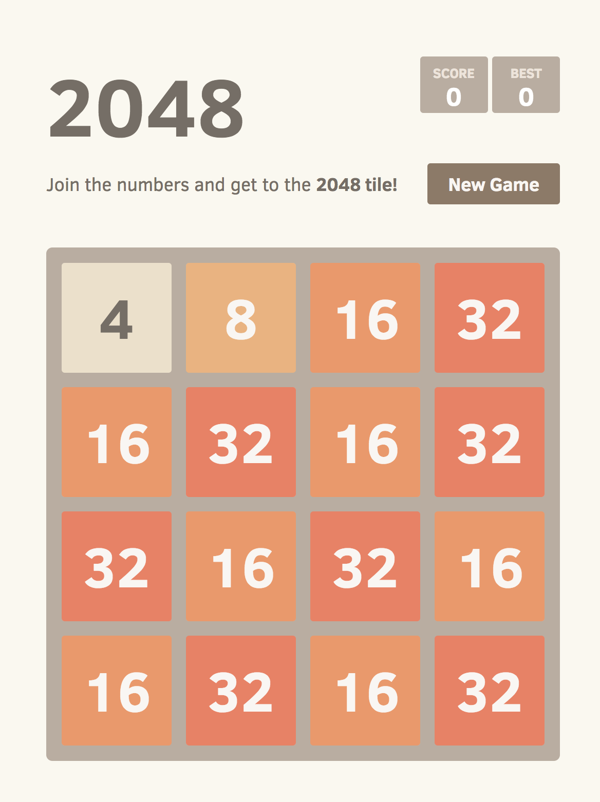
The explicit enumeration of states counts only states that can be reached in actual game play, but even with that restriction there are still some surprising states included in the count. For example, in the last figure above, the arc that shows the number of states with at most a 32 tile does not stop until tile sum 348. There are four states with tile sum 348 and no 64 tile, one of which I chose for the cover image of this post: 3

It contains seven 32 tiles and seven 16 tiles arranged in a nice striped pattern that makes it very difficult to merge any of them. I find it quite surprising that it’s possible to play to such a state without losing, and indeed it seems quite improbable, especially if one is ‘playing well’.
In the next post, we’ll explore what it means to ‘play well’ in a rigorous way by modeling the game of 2048 as a Markov Decision Process and finding an optimal policy for the 2x2 and 3x3 games — that is, we will find a strategy for playing those game that we can show mathematically to be at least as good as any other possible strategy.
Appendix A: Bit Bashing for Efficiency
Profiling the ruby code above revealed that most of the time was being spent on state manipulation — for example, moving tiles, counting available tiles, and reflecting or rotating states to find canonical states. Let’s see how we can speed it up.
The hexadecimal numerical representation for states has a convenient property: for the 4x4 board, we need to store 16 numbers, where each number takes 4 bits, for a total of 64 bits. Now that we all use 64-bit computers, this is an auspicious number: the whole board state can fit into a single 64-bit (8-byte) machine word. For example, the 4x4 state (which is a winning state, because it has a 2048 tile)

would be written 0x022b013020100000 in hexadecimal, or more clearly with the addition of line breaks to make a 4x4 grid:
022b
0130
2010
0000
With the state represented as a 64-bit integer, we can also implement many common manipulations on states very efficiently using bit mask and shift operations, often without loops 4. For example, the C++ function to reflect a 4x4 board state horizontally looks like:
uint64_t reflect_horizontally(uint64_t state) {
  uint64_t c1, c2, c3, c4;
  c1 = state & 0xF000F000F000F000ULL;
  c2 = state & 0x0F000F000F000F00ULL;
  c3 = state & 0x00F000F000F000F0ULL;
  c4 = state & 0x000F000F000F000FULL;
  return (c1 >> 12) | (c2 >> 4) | (c3 << 4) | (c4 << 12);
}
While initially quite opaque, all this is doing is shuffling bits around. The role of first bit mask, 0xF000F000F000F000ULL, becomes clearer if we omit the 0x and ULL, which just tell the compiler that this is non-negative 64-bit integer in hexadecimal, and again add line breaks to make a 4x4 grid:
F000
F000
F000
F000
The binary representation of the hexadecimal digit F is 1111, so the effect of this bit mask is to make c1 contain only the values in the first column of the board and zero bits everywhere else. The bit shift c1 >> 12 at the end of the function moves the first column 12 bits, which is to say three 4-bit cells, to the right, which makes it the last column. Similarly, c2 selects the second column, and c2 >> 4 moves it one cell to the right, and so on with the third and fourth columns to reverse the order of the columns.
Some functions take a bit more work to decipher. If you’re in the mood for a puzzle, here’s a function that counts the number of cells available (value zero) in a 4x4 state (you can find my explanation in comments here):
int cells_available(uint64_t state) {
  state |= (state >> 2);
  state |= (state >> 1);
  state &= 0x1111111111111111ULL;
  uint64_t count = ((state * 0x1111111111111111ULL) >> 60);
  if (count == 0 && state != 0) return 0;
  return 16 - count;
}
Profiling (with perf) showed that such tricks made a big difference — compared to the obvious implementations with arrays and loops, these functions require very few CPU instructions and contain few or no branches, which allows the CPU to keep its instruction pipelines full.
Appendix B: Layers and MapReduce for Parallelism
The next challenge is that we can’t keep the whole closed set in memory. To break up the state space into manageably sized pieces, we can use the following property of the game: The sum of the tiles on the board increases by either 2 or 4 with each move. This property holds because merging two tiles does not change the sum of the tiles on the board, and the game then adds either a 2 or a 4 tile. 1
This property is useful here because it means that we can organize the states into layers according to the sum of their tiles. We can therefore generate the whole state space by working through a single layer at a time, rather than having to deal with the whole state space at once.
To parallelize the work within each layer, we can use the MapReduce concept made famous by Google. The ‘map’ step here is to take one complete layer of states with sum \(s\) and break it up into pieces; then, for each piece in parallel, generate all of the successor states, which will have either sum \(s + 2\) or \(s + 4\). The ‘reduce’ step is to merge all of the pieces for the layer with sum \(s + 2\) together into a complete layer, removing any duplicates. The pieces with sum \(s + 4\) are retained until the next layer, in which states have sum \(s + 2\), is processed, at which point they will be included in the merge. This may be easier to see in an animation (made with d3):
In the map step for each piece, it is feasible to maintain the set of successor states in memory. To make the merge in the reduce step efficient, we want the map step to output a list of states for each piece in order by their state numbers so we can merge the pieces together in linear time. Here Google again comes to our aid: they have released a handy in-memory B-tree implementation that plays well with the C++ standard template library. B-trees are most commonly found in relational database systems, where they are often used to maintain indexes on columns. They keep data in order and provide logarithmic time lookup and also logarithmic time insertion — much better than logarithmic plus linear time insertion into a sorted list — with relatively little memory overhead.
To break the state space up into even smaller pieces, which reduces the amount of work we need to do in each merge step, we can exploit an another property of the game: the maximum tile value on the board must either stay the same or double with each move. This property holds because the maximum tile value never decreases, and when it does increase, it can only increase as the result of merging two tiles — that is, even if you have for example four 16 tiles in a row and you merge them, after one move the result is two 32 tiles, not one 64 tile.
Together with the property above, this means that from a list of states in which all states have tile sum \(s\) and maximum tile value \(k\), the generated successors will all fall into one of four pieces:
| Piece | 1 | 2 | 3 | 4 |
|---|---|---|---|---|
| Tile Sum | \(s+2\) | \(s+2\) | \(s+4\) | \(s+4\) |
| Max Tile Value | \(k\) | \(2k\) | \(k\) | \(2k\) |
There is a bit more bookkeeping to keep track of which pieces need to be merged together at each step, but it is basically the same idea. Here are the 57 states (excluding the ‘win’ and ‘lose’ states) for the 2x2 game to the 32 tile again, this time with the states grouped by tile sum and maximum tile value, here written \(s / k\):

For example, in the leftmost piece, both states have tile sum 4 and maximum tile value 2. The transitions from that piece are to pieces with tile sum either 6 or 8 and maximum tile value 2 or 4. Compared to the original diagram of these states without grouping, it’s also easier to see that you always transition to a state with a tile sum that is either 2 or 4 larger, like in the first post in this series.
Appendix C: Encoding and Compression
When working with billions or trillions of states, and each state takes 8 bytes, even fitting them all on disk is not trivial (or at least not cheap). To reduce the storage space required, and also the amount of input/output required, we can exploit the fact that the states are stored as sorted lists of integers — rather than storing each integer in full, we can store the differences between successive integers. These differences will generally be smaller than the integers themselves, so it is usually possible to store the differences in a smaller number of bytes. Using a variable-width encoding scheme to store the differences ensures that we use only the number of bytes we need. 5
For example, the list of states for the 4x4 game to the 2048 tile with tile sum 380 and maximum tile value 128 contains 21,705,361,721 states 2. At 8 bytes per state, that would be roughly 161GiB. However, with variable-width encoding, it takes only 35GiB — a compression factor of 4.6 — or about 1.7 bytes per state.
For longer term storage and transport over Internet, I also tried several compression programs on the variable-width encoded data. To evaluate the different programs, I used a smaller list of states with tile sum 260 and maximum tile value 32; it contained 30,954,422 states, which is about 1/700th the number in the 380/128 layer mentioned above, and it weighed in at 64MiB after variable-width encoding. For each of the programs, and for each of their supported compression levels, I measured the elapsed time for compression and the resulting compressed size using this smaller list of states.
Three programs emerged on the resulting Pareto frontier: Facebook’s Zstandard, Google’s Brotli and 7-zip. After scaling size and time up by a factor of 700 to estimate performance on the larger 380/128 layer, the frontier looks like:

Here closer to the origin is better; we see Zstandard performing best for relatively fast and light compression, and 7zip performing best for relatively slow and heavy compression. From the graph, we can see that Zstandard at compression level 11 is fairly close to the origin, and it turned out to minimize the particular linear cost function that I used. The results on the smaller layer suggested that Zstandard level 11 would reduce the 380/128 layer from 35GiB to about 10GiB. In fact, it did much better: it reduced it from 35GiB to 3.8GiB, for another factor of 9.2, or about 1.5 bits per state. I think that’s quite remarkable.
Thanks to Hope Thomas for reviewing drafts of this article.
If you’ve read this far, perhaps you should follow me on twitter, or even apply to work at Overleaf. :)
Footnotes
-
This property was called called Property 3 in the previous post, and we also used it anonymously in the first post. It is a very useful property. ↩ ↩2
-
These figures come from the one month build on the full 4x4 game, which used an additional technique for reducing the size of the state space: for each state, it looked one move ahead to see whether the next move was a definite win or a definite loss; if it was, the state was collapsed to a special ‘one move to win’ or ‘one move to lose’ state. This technique was not very effective, however, because states that are close to a loss tend to have few very successors anyway, and because win states only occur much later in the game, and the enumeration process never reached a win state. I therefore haven’t included it in the main body of the article, but the code is here. The state counts mentioned in this article for the partial enumeration of states with the 4x4 board to the
2048tile are slightly reduced compared to what they would be without this technique, but only slightly. ↩ ↩2 -
In case you are wondering, I faked that screenshot; I didn’t actually play the game to that state! ↩
-
The bit bashing techniques used here are based mainly on 2048-ai by Robert Xiao and 2048-c by Kuang-che Wu, with some help from Bit Twiddling Hacks by Sean Eron Anderson. The original motivation for 2048-ai and 2048-c was to allow real time search for 2048 AI bots. ↩
-
Variable width encodings are most commonly encountered in the UTF-8 character encoding for unicode, which you are using as you read this webpage. They are also sometimes used for storing integer primary key indexes in some databases, which also face the problem of efficiently storing large lists of sorted integers. The implementation used here is libvbyte from Christoph Rupp, based on work by Daniel Lemire. ↩